Capacitive Soil Moisture Sensor: How it Works
 Akuasense

A capacitive soil moisture sensor is an instrument that measures the soil’s dielectric permittivity in order to estimate its volumetric water content; the Akuasense soil moisture probes use the 100+ MHz technique. In this document, sensor refers to the capacitive measuring device and probe to the complete system (sensor, PVC tube, electronics).
Key points
- Akuasense probes use a 100+ MHz capacitive measurement to continuously monitor soil moisture.
- The physical quantity actually measured is the soil’s apparent dielectric permittivity, denoted .
- The volumetric water content is derived from using a dielectric mixing model suited to sandy soils (the CRIM model).
- The strong permittivity contrast between air, mineral soil and free water makes the measurement highly sensitive to moisture variations.
- In coarse-textured soils, the dielectric measurement offers high accuracy and excellent reproducibility for agronomic management.
General operating principle
The sensor is a capacitive measuring instrument operating at a frequency of 100+ MHz.
It is installed inside a PVC tube and enables soil moisture monitoring.
Measured quantity
The probe measures the apparent dielectric permittivity of the medium surrounding the tube, denoted:
from which the volumetric water content is derived, defined as the ratio of the water volume to the total soil volume:
Units and symbols:
- : volumetric water content [ or %]
- : volume of water contained in the sample []
- : total volume of the soil sample []
Dielectric contrast
The measurement relies on the large difference in permittivity between the soil constituents (dimensionless values):
| Medium | Dielectric permittivity (approx.) |
|---|---|
| Air | |
| Mineral soil (sand / clay) | to |
| Free water |
Consequence: a minor change in water content causes a major change in the overall permittivity.
Physical basis: why the square root of permittivity?
This section explains why the probe’s response is proportional to the square root of the permittivity, also called the refractive index.
Refractive index
For non-magnetic materials (the case of soil):
- : refractive index of the medium [dimensionless]
- : relative dielectric permittivity [dimensionless]
Propagation speed
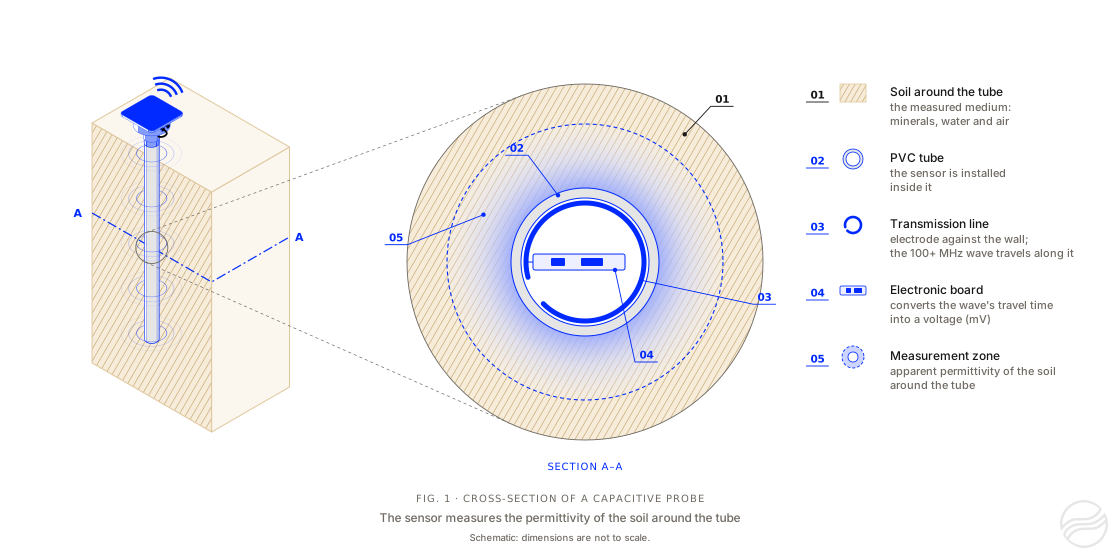
Figure 1. Cross-section of an Akuasense capacitive probe. The sensor is installed inside a PVC tube. The electronic board sends a wave along the transmission line, which lies against the inner wall of the tube, and converts the travel time of this wave into a voltage. This travel time depends on the apparent dielectric permittivity of the soil around the tube, in the measurement zone.
The sensor emits an electromagnetic wave along the transmission line.
The speed of this wave in the soil is:
- : wave speed in the medium []
- : speed of light in vacuum ()
Propagation time
For a fixed transmission line length , the propagation time is:
Substituting , we obtain:
- : wave travel time [ or ]
- : length of the transmission line (electrode) []
Physical conclusion
- and are constant.
- The measured time is proportional to .
Signal conversion chain
From raw signal (mV) to permittivity
The electronics convert the wave’s propagation time into a voltage by measuring the phase shift between a source wave and the propagated wave.
The relationship between the refractive index and the measured signal is then modeled as:
- : probe output signal [millivolt]
- : slope coefficient (sensitivity) []
- : offset constant [dimensionless]
The coefficients and are determined during calibration.
Application to sandy soils
In coarse-textured soils (sands, silty sands), the interaction between water and the solid matrix is purely mechanical, which makes the dielectric measurement extremely accurate.
The mixing rule
The CRIM model (Complex Refractive Index Model) considers that the total refractive index measured by the probe is the weighted sum of the indices of each soil component:
Where (units and definitions):
- : volumetric water content []
- : overall measured refractive index [dimensionless]
- : refractive index of water ()
- : refractive index of quartz / sand ()
- : refractive index of air ()
- : soil porosity []
- : volume fraction of the solid phase []
Expansion and simplification
Since the refractive index of air , the equation becomes:
Isolating the water content ()
Grouping the terms containing on one side of the equation:
Final equation for the water content ()
The equation used to directly compute the volumetric water content is therefore:
FAQ: Understanding capacitive measurement
Why use a frequency of 100+ MHz for moisture measurement?
Using high frequency (100+ MHz) in Akuasense probes minimizes the influence of soil salinity and texture on the measurement. At this frequency, the effect of ionic conduction losses is reduced, ensuring that the variation of the dielectric permittivity is mainly due to the presence of free water.
What are the advantages of the CRIM model for sandy soils?
The CRIM model (Complex Refractive Index Model) is particularly effective in coarse-textured soils because it treats the soil as a simple multiphase mixture. In sand, the absence of surface electrical charges (unlike clays) allows a nearly perfect linearity between the measured refractive index and the volumetric water content .